Unlocking Marketing ROI: How Budget Phasing Algorithms Revolutionize Marketing Mix Modeling Accuracy

The perennial challenge of accurately measuring the return on marketing investment (ROI) has long been a complex puzzle for growth strategists. In recent years, Marketing Mix Modeling (MMM) has experienced a significant resurgence, driven by advancements in open-source tools such as Meta’s Robyn, Google’s Meridian, and PyMC-Marketing from PyMC Labs. While running an MMM has become more accessible than ever, the crucial question of trust and reliability remains paramount. A seminal 2017 paper from Google, "Challenges and Opportunities in Media Mix Modeling," laid bare the persistent issues plaguing MMM accuracy, many of which stem from the inherent variations missing in marketing spend data. This article delves into these challenges, explores the limitations of current solutions like incrementality testing, and introduces a promising new approach: budget phasing algorithms, designed to inject the necessary variations into marketing plans and dramatically improve MMM’s predictive power.

The Persistent Challenges in Marketing Mix Modeling

Google’s 2017 analysis highlighted three core problems that significantly undermine the effectiveness of MMM. These issues arise from different types of variation that are often absent from historical marketing spend data. The industry’s primary response over the past decade has been to lean on incrementality testing, increasingly used to calibrate MMMs. While this represents genuine progress, incrementality tests typically analyze one channel at a time and can require months to yield reliable impact data. Furthermore, a 2026 Recast study revealed that a significant percentage of open-source geo-testing tools (14-30%) report false lifts, casting doubt on their standalone accuracy.

The underlying issue, as identified by Google and further explored in this analysis, is that the data used for MMM often lacks the dynamic variation needed for robust modeling. Specifically, three critical types of variation are frequently missing:

• Independent Channel Movement: When marketing channels are budgeted and executed in lockstep, it becomes exceedingly difficult for an MMM to isolate the unique impact of each individual channel. If TV, Meta, Search, and TikTok all increase spend simultaneously, the model struggles to disentangle which channel was responsible for driving sales uplift.
• Spend Variation Relative to Demand: Marketing budgets are often planned in alignment with anticipated demand. When demand rises, so too does marketing spend. This co-movement creates "omitted variable bias," where the MMM inadvertently attributes sales increases to marketing channels, even when the primary driver was an underlying surge in consumer interest.
• Sufficient Spend Levels for Response Curve Identification: Accurately modeling how a channel’s effectiveness changes with increased spending (saturation) or how long its impact lingers (adstock) requires data points at varied spend levels. If spend remains within a narrow range, the model cannot reliably discern these crucial response curve shapes.

The common thread running through these problems is a lack of strategically varied marketing spend. The central hypothesis explored in this research is whether a budget phasing algorithm can proactively introduce these necessary variations into a planned marketing budget, thereby enhancing the quality of data available for MMM.

Simulating the Ground Truth: A Data-Driven Approach

To rigorously test the efficacy of budget phasing algorithms, a controlled environment with a known ground truth is essential. This research employs a data-generating process (DGP) to simulate marketing spend and revenue over a three-year period. This allows for a direct comparison between the model’s estimates and the actual simulated outcomes, providing an unbiased assessment of the algorithm’s impact. This methodology is standard practice for validating MMM performance, but here it serves to specifically evaluate the influence of a budget phasing strategy.

Step 1: Simulating Marketing Spend and Demand Dynamics

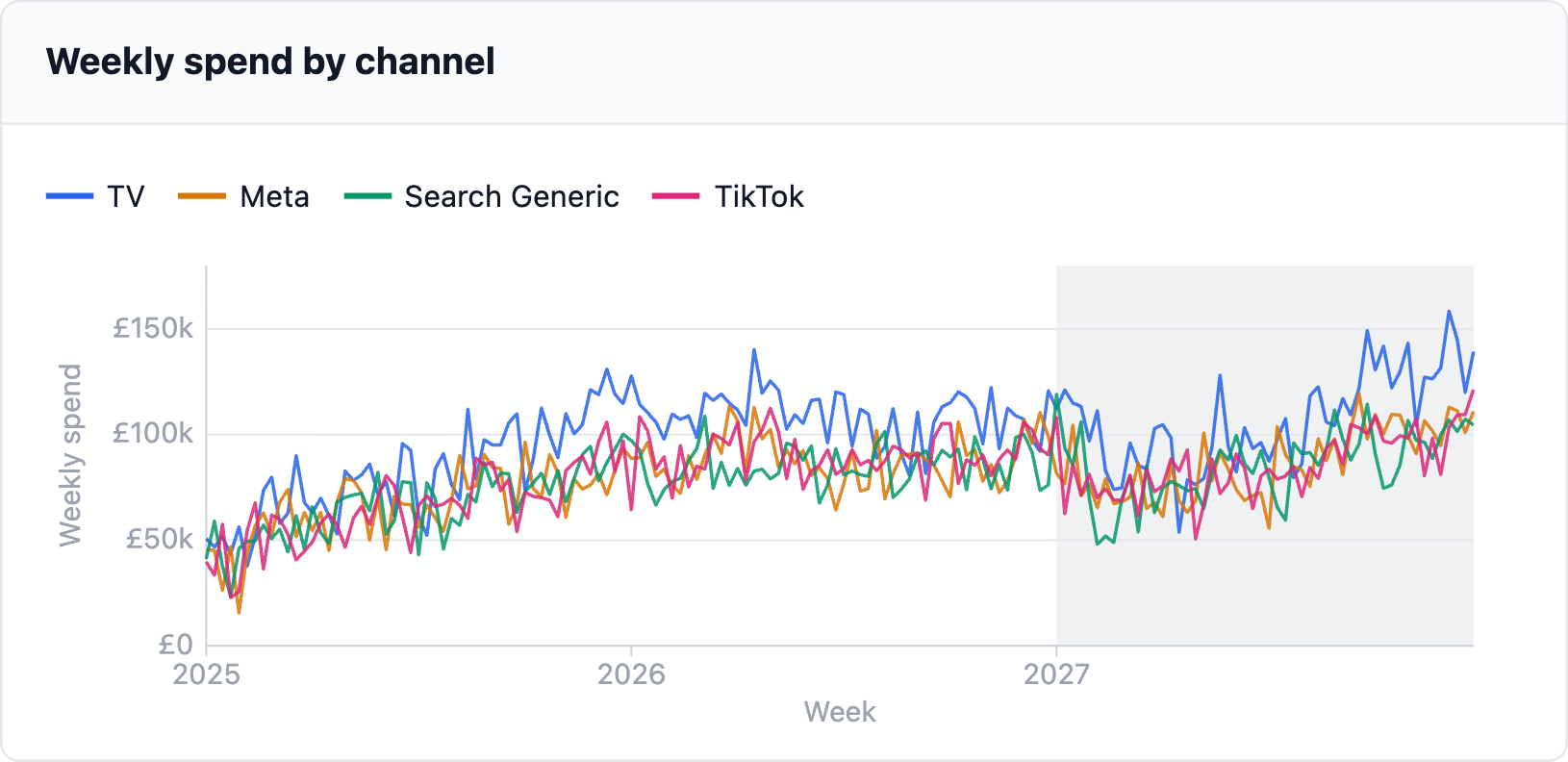
The simulation begins by generating three years of weekly spend data across four key marketing channels: Television (TV), Meta, Search Generic, and TikTok. While most real-world scenarios involve a broader portfolio of channels, these four are selected for illustrative purposes, with the understanding that the methodology can scale to 10-15 channels. The three-year timeframe is chosen to balance the need for sufficient historical data with the imperative of maintaining recent insights, a common practice in MMM.

A crucial aspect of the simulation is the inherent correlation between these channels. In this model, all channels share an underlying signal, resulting in a correlation coefficient of 0.7. This high correlation is realistic, as budget planning often aligns with overarching demand forecasts, leading to synchronized spending patterns across platforms. The simulation also incorporates an upward trend in this shared signal, leading to a gradual increase in spend over the three years. It is important to note that in a real-world application, marketers would provide their actual spend data for the past two years and their planned budget for the upcoming year, which would then constitute the three-year window for MMM training.

Beyond marketing spend, underlying demand—the volume of purchases irrespective of advertising—also plays a pivotal role in sales. Because budgets are frequently planned around demand forecasts, demand itself tends to move in tandem with spend. This co-movement is a primary source of selection bias in MMM. Since demand is not directly observable, it is constructed in the simulation to move with spend, exhibiting a correlation of 0.65. This figure is an assumption, as actual spend data alone cannot definitively reveal the true demand correlation. The simulation posits that spend accounts for slightly over half of the demand in this scenario, with the remainder following one of five distinct patterns (e.g., steady growth, strong yearly cycles). Marketers would typically identify the pattern that best describes their sales behavior, excluding marketing influences.

Step 2: Defining Marketing Channel Responses

Before generating sales figures, the simulation establishes the response functions for each marketing channel. This involves defining three key parameters:

• Marginal Return: This represents the revenue generated by an additional unit of spend at the channel’s planned weekly expenditure. For instance, in the scenario used, TV has a marginal return of £0.50 per £1 spent, while Search Generic offers £1.50.
• Saturation Curve: This parameter dictates how quickly the effectiveness of additional spend diminishes. A saturation exponent of 1.0 indicates a linear relationship, whereas lower values signify a faster rate at which extra spending yields diminishing returns.
• Adstock Decay: This measures the carry-over effect of advertising, indicating how long an ad’s impact persists after the week it airs. For example, TV has a 0.50 adstock decay, meaning half of its effect extends into the following week, while Search Generic has a 0.10 decay.

The simulation uses plausible values for these parameters to create a realistic scenario. In practice, these values would ideally be derived from the marketer’s existing MMM results, creating a somewhat circular but necessary process to generate realistic sales data where the true response is known. This allows for an accurate measurement of how correlated spend impacts model accuracy and the extent to which budget phasing can rectify these issues.

The table below outlines the specific parameters used in the simulation:

Channel	Marginal Return (£ per extra £1)	Saturation	Adstock
TV	0.50	0.60	0.50
Meta	1.00	0.75	0.30
Search Generic	1.50	0.90	0.10
TikTok	1.20	0.70	0.20

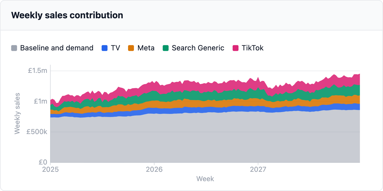
A baseline sales figure, representing sales with no marketing activity, is set at 70% of total sales. All variance and bias figures presented in this analysis are conditional on these inputs, illustrating what a model might misinterpret under these specific simulated conditions.

Step 3: Generating Sales and Revenue

With all components defined, the simulation generates weekly sales/revenue using the following formula:

Sales = Baseline + (Demand Coefficient * Demand) + Σ (Channel Contributions) + Noise

The resulting decomposition chart visually represents the drivers of sales each week, serving as the ground truth against which MMM estimates can be compared. This detailed simulation process provides a robust foundation for analyzing the limitations of traditional MMM and the potential of budget phasing.

The Three Pillars of MMM Misinterpretation

The simulated data now allows for an examination of the core problems that can lead MMMs astray. The analysis focuses on three critical areas: variance, bias, and identifiability.

Problem 1: Variance in Estimates

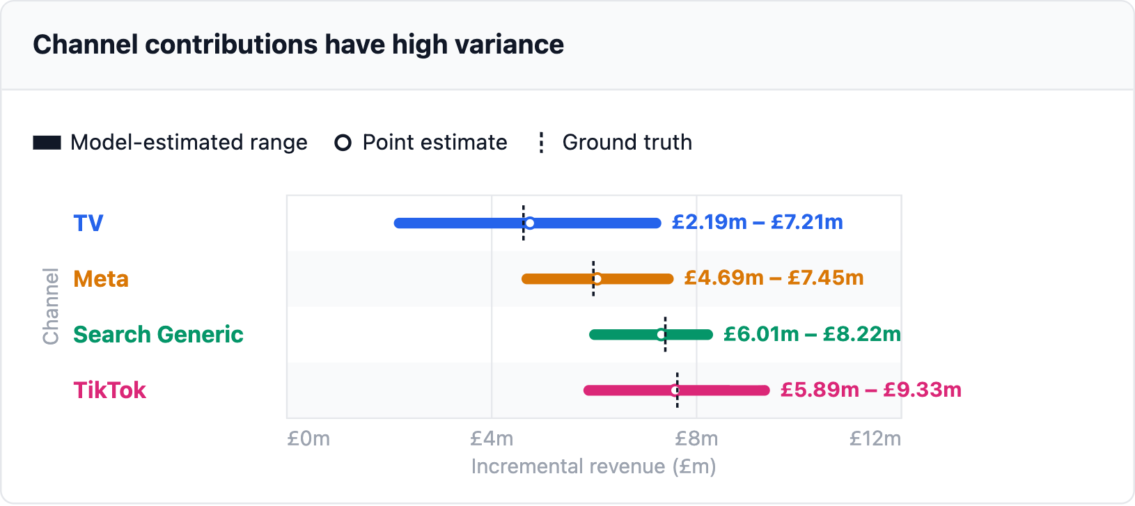
To assess variance, 50 different sales series are generated from the DGP, each differing only in the random noise component. The marketing spend, response functions, and demand remain constant across these simulations. An MMM is fitted to each series, assuming accurate demand proxies and known curve shapes. The objective is to observe how much the estimated incremental revenue for each channel fluctuates across these 50 refits, particularly when compared against the known ground truth.

The results, visualized in a forest plot, reveal substantial ranges for the estimated incremental revenue for each of the four channels. This wide spread indicates high variance. Notably, any of the four channels could appear to be the highest revenue driver based on a single refit. This is not necessarily bias; with correlated channels, the regression can still converge on the true average impact over many runs. However, with only three years of weekly data, there is limited independent movement per channel, meaning any single MMM fit could land anywhere within this broad range, leading to unreliable conclusions.

Problem 2: Bias in Point Estimates

Bias is examined by introducing a more realistic scenario where the MMM receives a demand proxy instead of the true, simulated demand. To account for the variability in demand proxies, 100 different versions of demand and its proxy are generated. For each of these, 50 sales simulations are run, resulting in 5,000 refits. The average estimated incremental revenue is then compared to the ground truth.

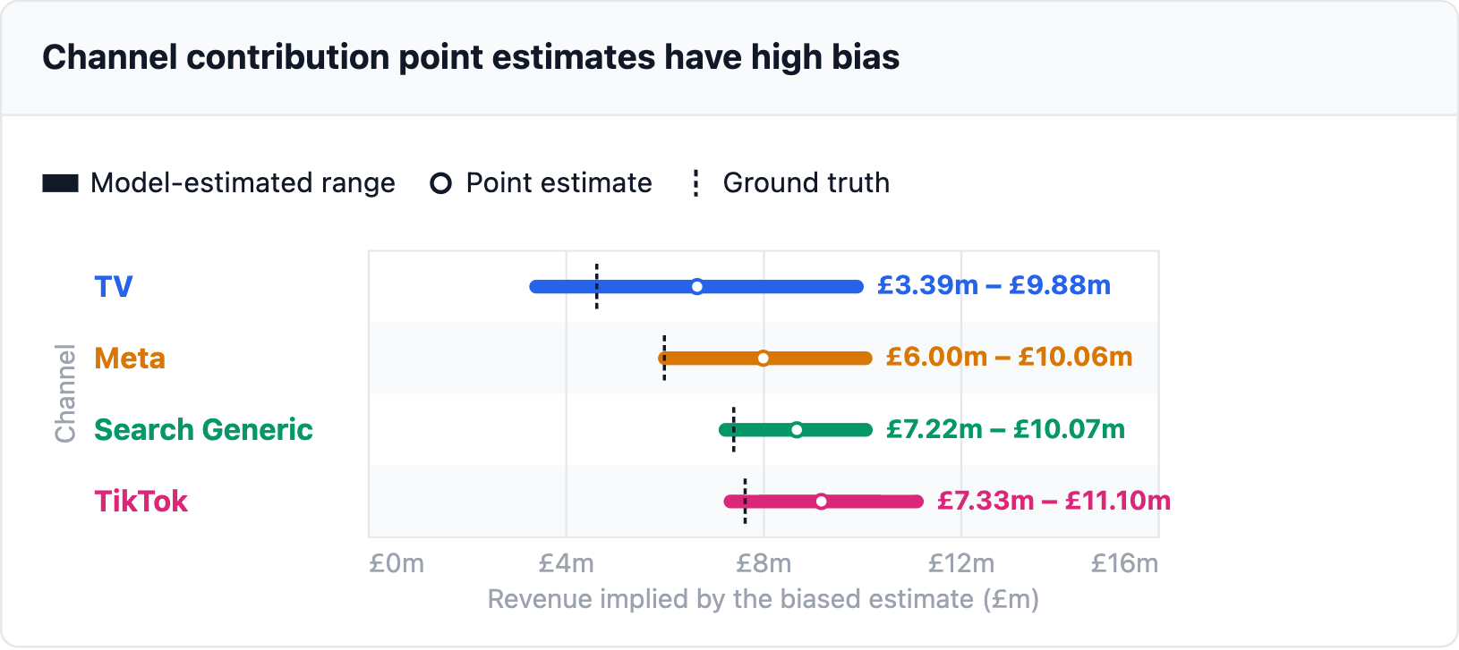
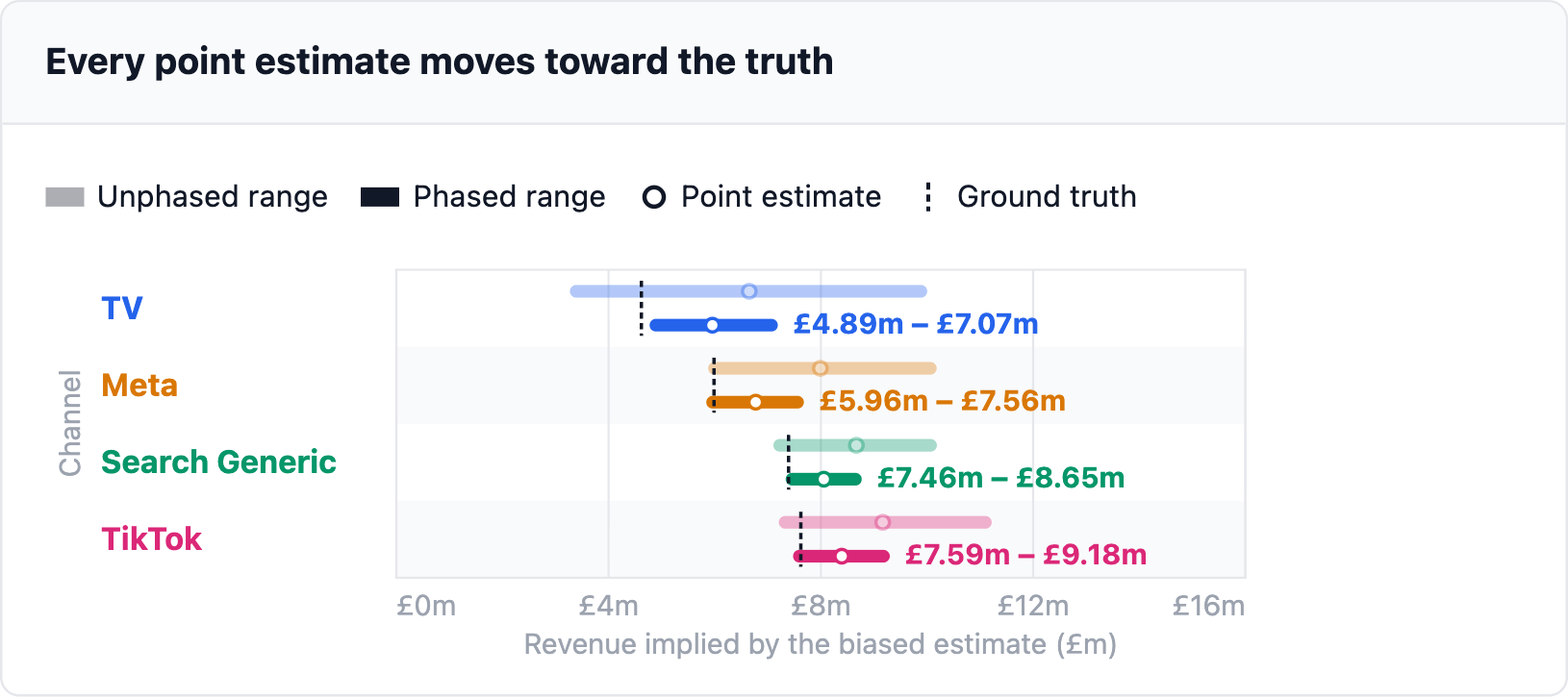
The forest plot for bias starkly illustrates the problem. The point estimates for every channel consistently sit above the ground truth: TV by 44%, Meta by 33%, TikTok by 20%, and Search Generic by 17%. This upward bias is driven by the co-movement of spend and demand. When demand increases sales, spend also increases. The MMM, lacking the true demand signal, incorrectly attributes a portion of these sales to the marketing channels. This "omitted variable bias" does not diminish with more data; refitting the same mis-specified model on more weeks merely tightens the estimate around the wrong number.

Problem 3: Identifiability of Response Curves

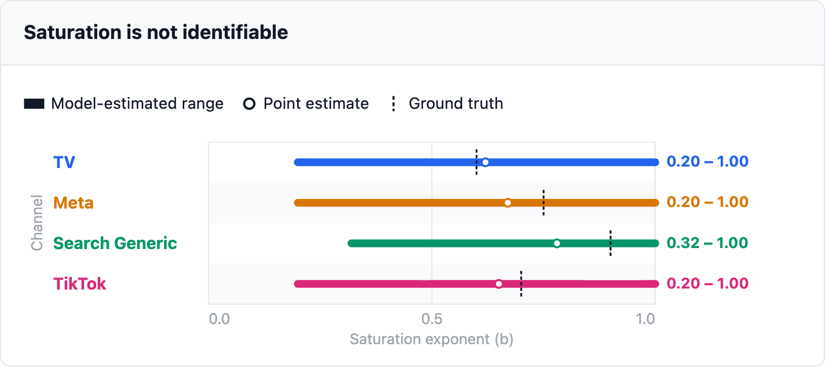
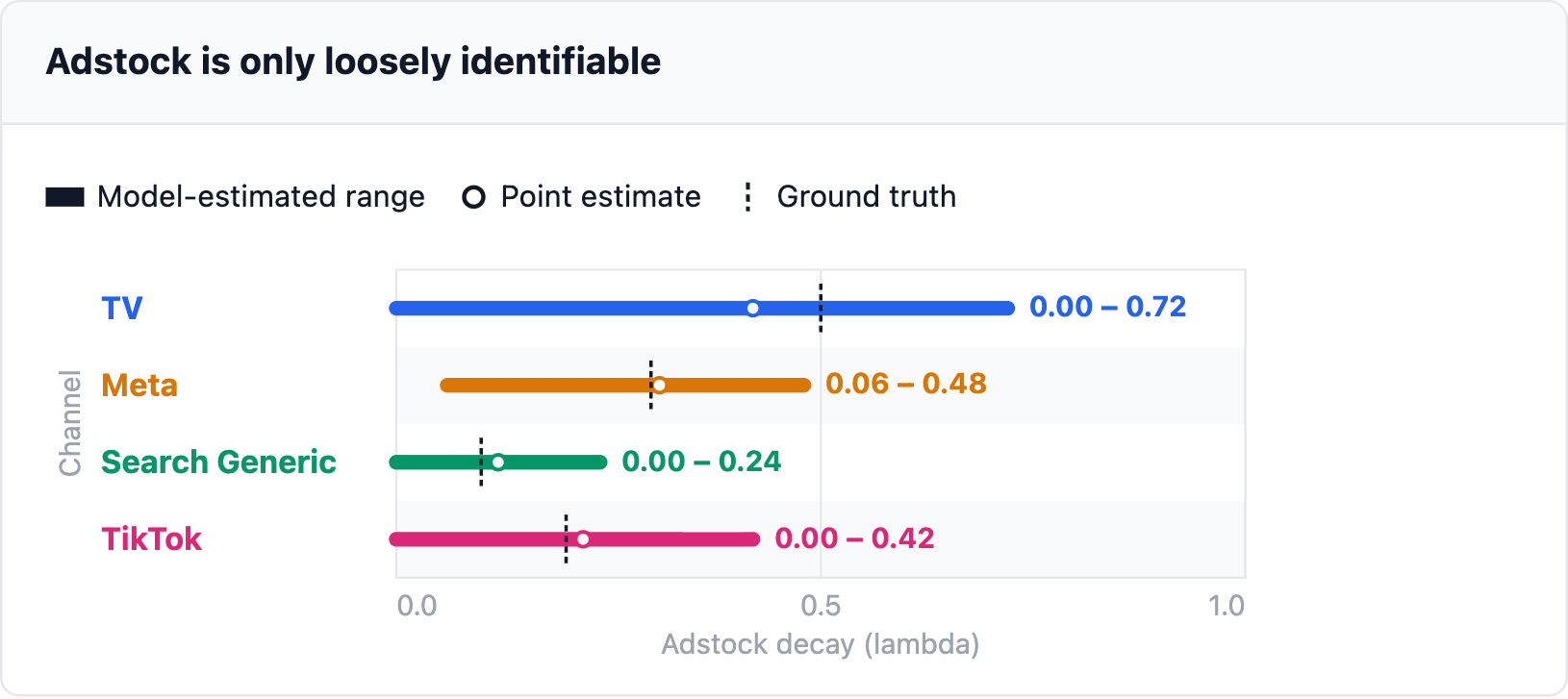
The ability of an MMM to accurately identify the saturation curves and adstock decay rates of marketing channels is crucial for understanding their long-term effectiveness. To test identifiability, 50 sales series are generated with fresh noise, and the model receives the true demand. For each channel, its saturation exponent and adstock decay are systematically varied across a plausible range (saturation: 0.20-1.00; adstock: 0.00-0.90), and the combination that best fits the data is retained. The spread of these "best fits" across the 50 series reveals the model’s identifiability.

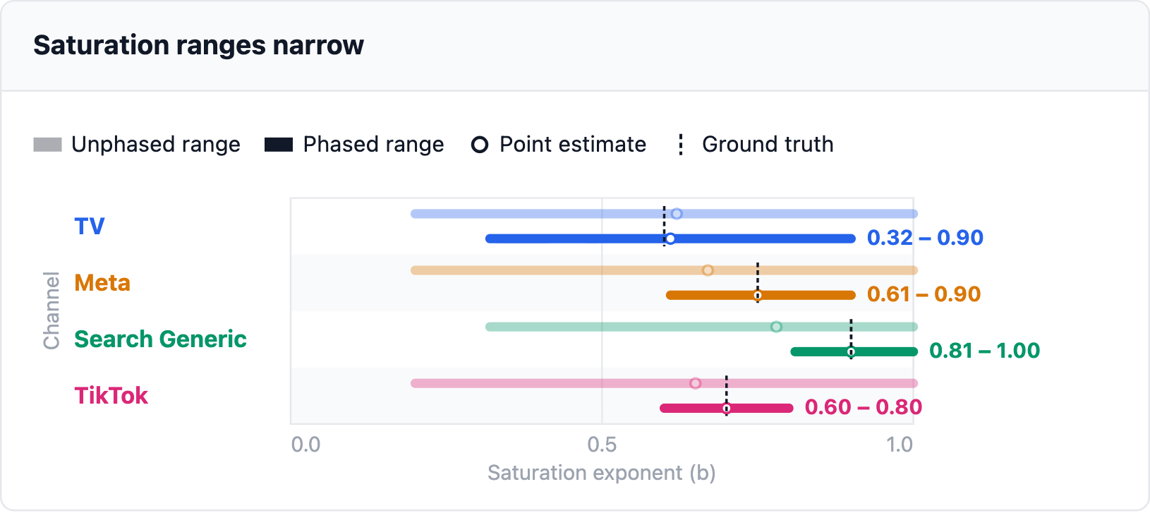
Saturation proves to be particularly problematic. For three of the four channels, the recovered range spans the entire tested spectrum (0.20 to 1.00). This means the model struggles to differentiate between a curved response and a linear one because it lacks observations at sufficiently distinct spend levels. When all channels move together, a straight line and a curve can fit the data similarly well. Adstock is somewhat better but still exhibits wide ranges, with many channels showing a recovered decay that reaches zero, implying ads stop working the week they run—a scenario that contradicts practical experience. For example, TV’s true decay of 0.50 has a recovered range from 0.00 to 0.72.

The common industry response to these issues—tinkering with model priors, transformations, or specifications—often proves ineffective. The fundamental problem lies not with the model’s architecture but with the data’s inherent limitations. When channels consistently move in unison, no estimation method, however sophisticated, can reliably disentangle their individual contributions.

The Root Cause: Channels That Never Move Alone

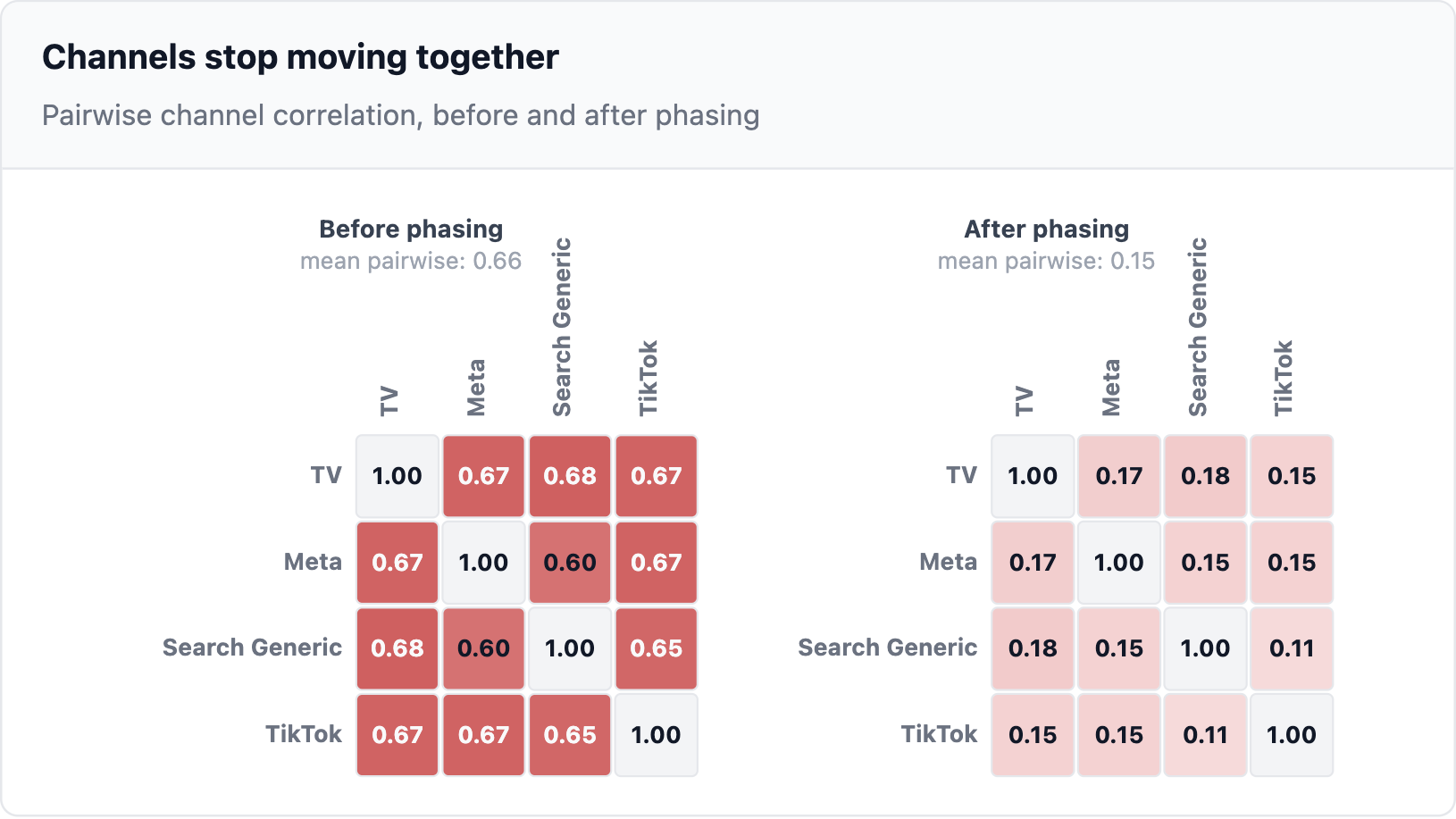
The challenges of variance, bias, and identifiability are intrinsically linked to the correlated movement of marketing channels. In the simulated scenario, budgets for TV, Meta, Search Generic, and TikTok are set within the same planning cycle, leading to a strong correlation (between 0.60 and 0.68 for every pair).

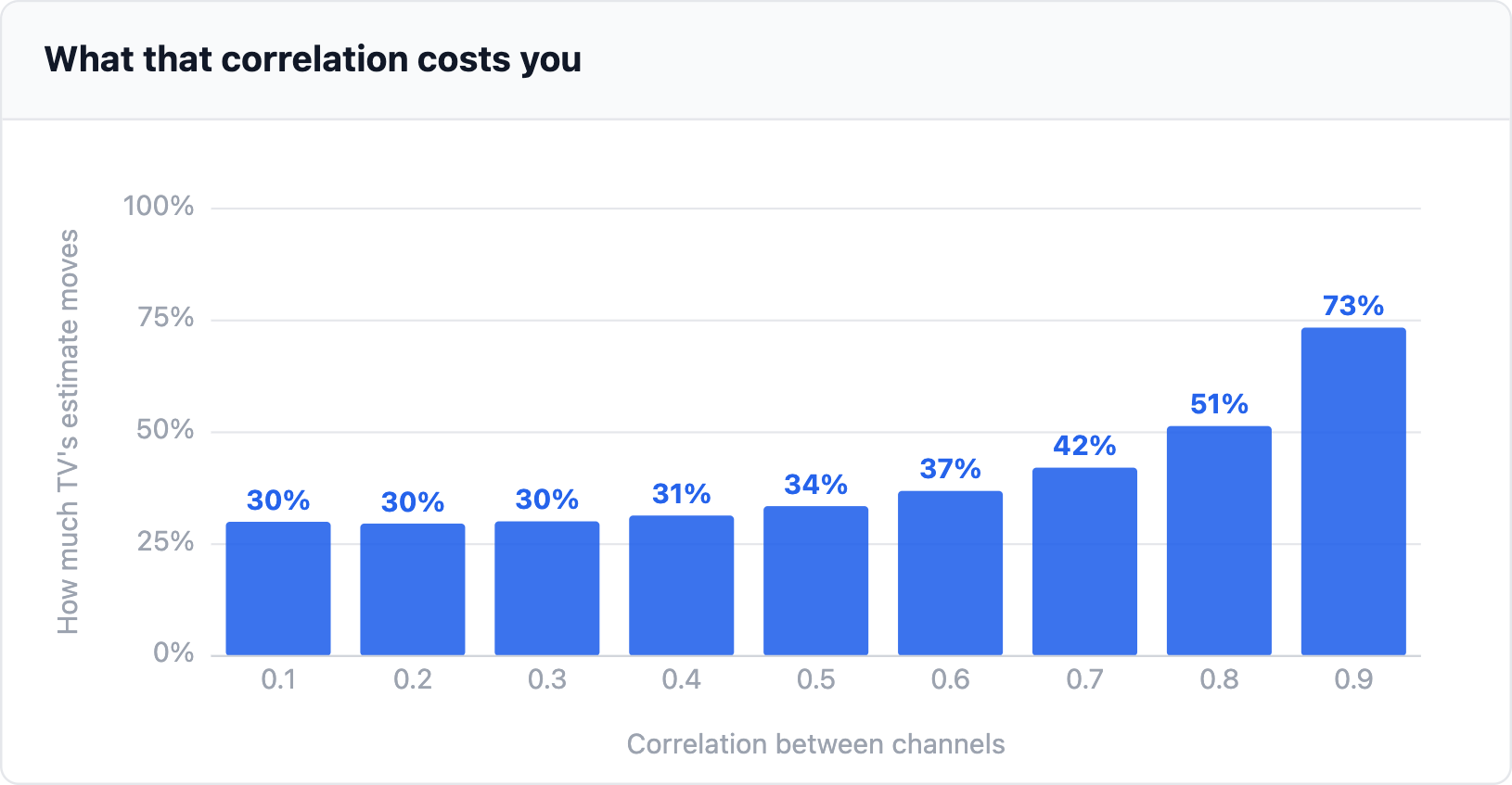
To quantify the impact of this correlation, the variance measure from Problem 1 is re-evaluated across a range of correlations from 0.1 to 0.9, while keeping other factors constant. The coefficient of variation for TV’s estimated incremental revenue (how much its estimate fluctuates relative to its mean) is tracked. Even with completely independent channel movements, some variance (around 30%) is expected due to sales noise and data limitations. However, as correlation increases, so does the variance. At the simulated 0.7 correlation, variance rises to 42%, and at 0.9, it escalates to 73%.

Bias exhibits a different dependency, being more sensitive to the strength of the link between spend and demand rather than inter-channel correlation. Holding channel correlation at 0.7 and varying the spend-demand link reveals that even a weak link (0.1) results in TV’s estimate being 11% too high. At the simulated 0.65 link, this bias reaches 44%, and at a strong 0.86 link, it soars to 89%.

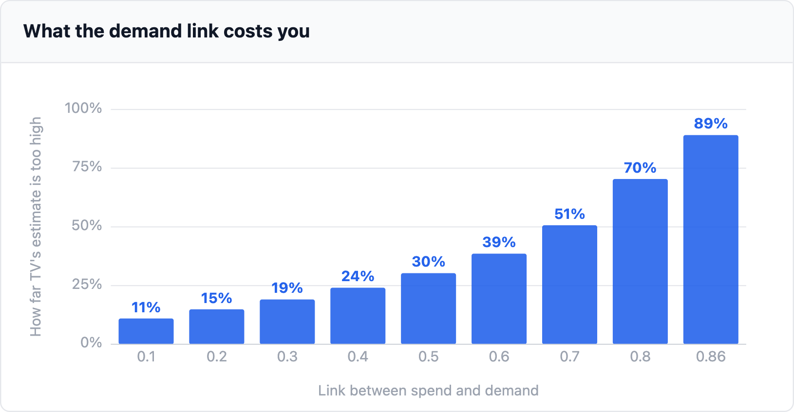
The problems of adstock and saturation have a distinct cause. Adstock requires observing sustained periods of spend to detect carry-over effects, while saturation needs spend data at clearly different levels. The lack of these specific variations in correlated spend patterns exacerbates these identifiability issues. The core takeaway is that the data, as it is typically collected, is not designed to answer the critical questions that MMMs aim to address.

A Smarter Approach: Budget Phasing Algorithms

The solution to these pervasive MMM challenges does not lie in more complex models or additional AI agents. Instead, it resides in optimizing the input data itself. A budget phasing algorithm can strategically alter the timing of marketing spend, injecting the necessary information into the data without increasing the overall budget or fundamentally changing the media mix. The goal is to create spend patterns where each channel moves independently of demand and at varied levels, held for sufficient durations to allow the MMM to learn.

While the concept of intentionally varying spend is not new—vendors like Recast advocate for it, and "go-dark" tests have been employed for years—the precise "how much," "which channel," and "what is the return" have been less clear. This section explores various phasing strategies and their effectiveness.

The Mechanics of Budget Phasing

Effective budget phasing must address the distinct data requirements identified earlier:

• Variance Reduction: Requires channels to move independently of each other and of demand.
• Bias Reduction: Necessitates spend variations not directly driven by demand fluctuations.
• Identifiability Improvement: Demands spend at a range of levels and for varying durations.

Evaluating Phasing Strategies

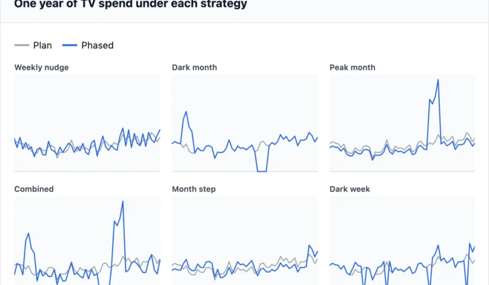
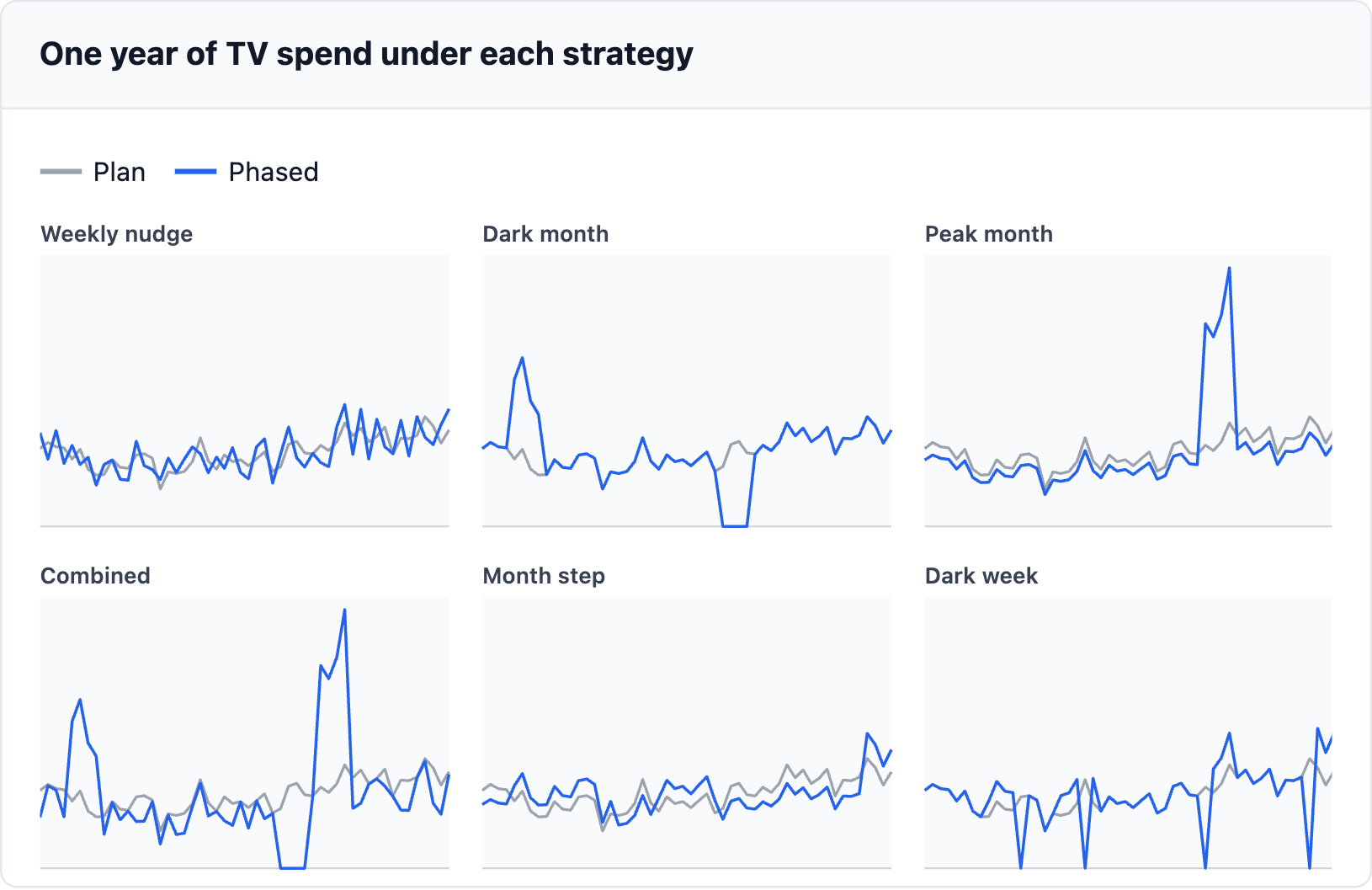
Six distinct phasing strategies are tested, starting with three foundational approaches, each targeting one of the core MMM problems. A fourth strategy combines these elements, and two lighter alternatives are also assessed. All strategies maintain each channel’s annual budget, with variations occurring within the year.

The strategies include:

1. Unphased: The baseline plan with no strategic timing changes.
2. Weekly Nudge: Small, consistent weekly adjustments to spend (e.g., +/- 10%).
3. Dark Month: Entirely pausing spend for one month for a specific channel.
4. Peak Month: Concentrating additional budget into a single month for a specific channel.
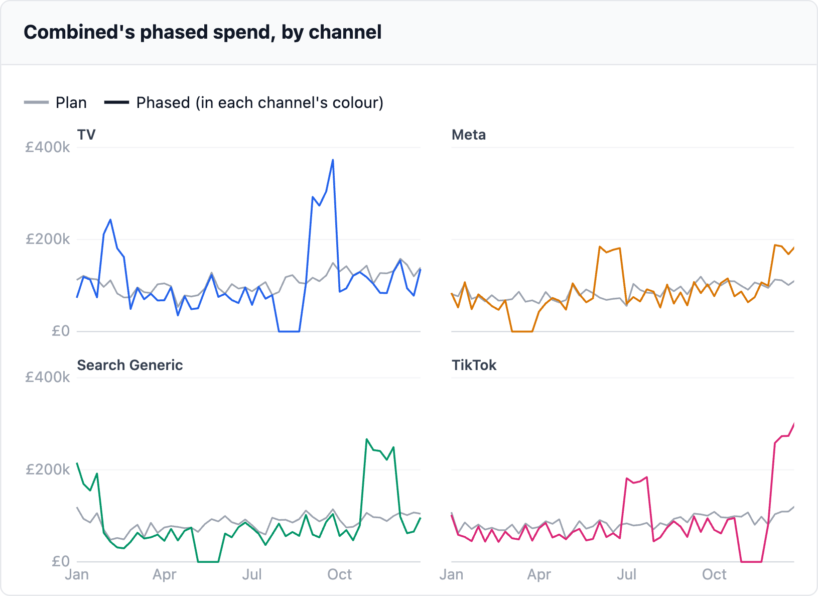
5. Combined: A comprehensive strategy integrating elements of weekly nudges, dark months, and peak months across channels.
6. Month Step: Shifting budget between months without drastic changes.
7. Dark Week: Short, intermittent pauses in spending.

The Verdict: Which Strategy Delivers?

Each strategy is evaluated against the MMM challenges of variance, bias, saturation identifiability, and adstock identifiability. The "Combined" strategy emerges as the most effective across all diagnostic measures. It significantly reduces variance (from 0.23 to 0.07) and bias (from 28.8% to 15.3%), while substantially improving the identifiability of saturation (from 0.77 to 0.31) and adstock (from 0.45 to 0.18).

However, this superior performance comes at a cost. The "Combined" strategy leads to a 3.42% reduction in planned revenue compared to the unphased plan. The "Dark Month" strategy presents a compelling alternative, achieving 92% of the variance gain and 71% of the bias gain of the "Combined" strategy, albeit at a lower cost (1.82%). The "Weekly Nudge" strategy is the least effective, with "Month Step" outperforming it on variance and bias.

The cost of these strategies is a critical consideration. In the simulated scenario, the "Combined" strategy incurs a revenue reduction of approximately £0.9 million on a £25.6 million planned revenue, equating to 3.42% of the channels’ driven revenue. This cost is influenced by the saturation curves, which are themselves subject to the identifiability issues. If saturation curves are less pronounced, the cost of phasing is lower.

The Impact of the Combined Strategy

Focusing on the "Combined" strategy, its implementation leads to a profound transformation of the spend data.

Reimagining the Spend Schedule

The "Combined" strategy typically involves four dark weeks and two months of heightened spend per channel within the planning year. Crucially, no two channels are scheduled for dark weeks in the same month. This approach ensures that the annual budget remains constant, but the weekly and monthly allocations are strategically adjusted.

Decimating Channel Correlation

A key outcome of the "Combined" strategy is the dramatic reduction in inter-channel correlation. Before phasing, the mean pairwise correlation between channels stands at 0.66. After implementing the "Combined" strategy, this correlation plummets to an average of 0.15, with specific pairs falling as low as 0.11. This disentanglement of channel movements is fundamental to improving MMM accuracy.

Quantifiable Improvements

The impact on the core MMM challenges is substantial:

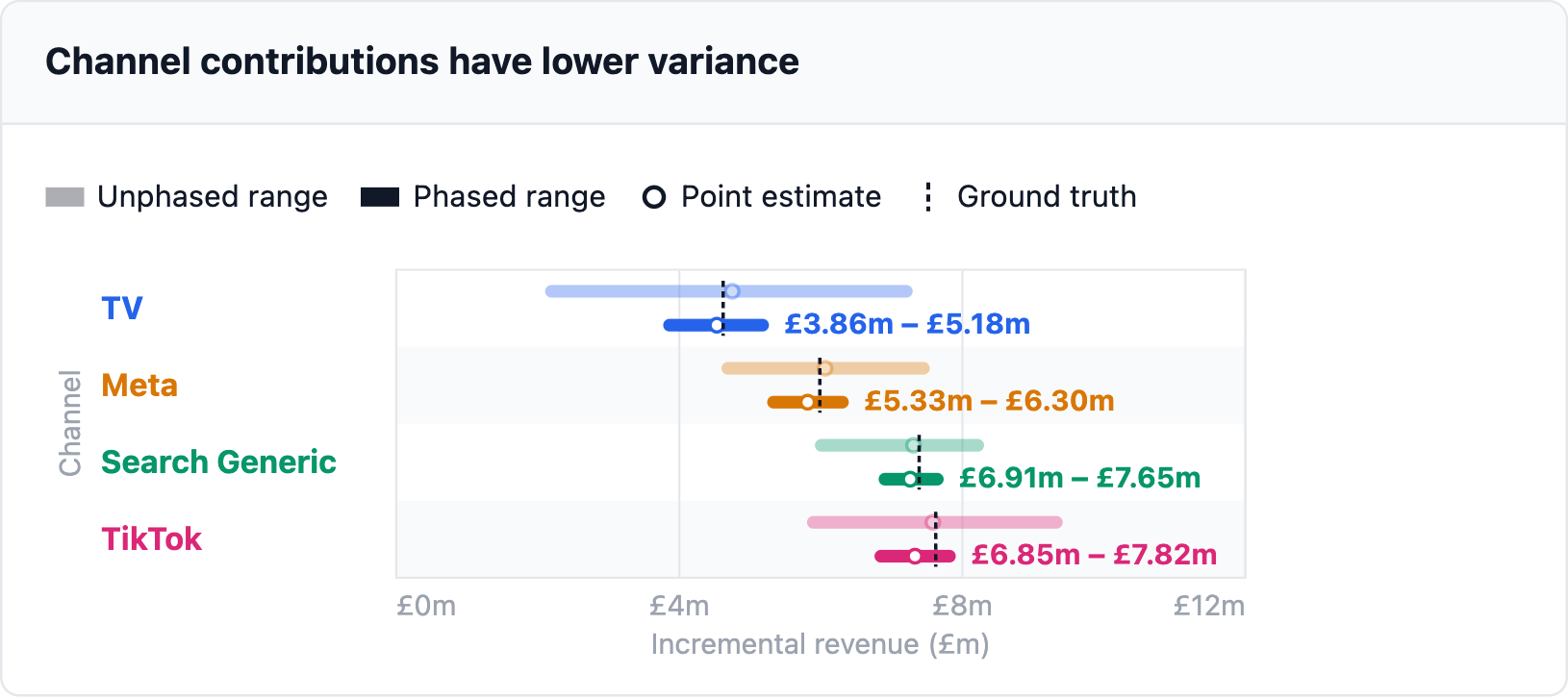
• Variance Reduction: The range of estimated incremental revenue narrows significantly for every channel, with improvements ranging from 65% for Meta to 74% for TV.
• Bias Reduction: Point estimates for all channels move closer to the ground truth. TV’s bias decreases from 44.0% to 29.0%, Meta’s from 33.5% to 13.1%, TikTok’s from 20.2% to 10.1%, and Search Generic’s from 17.3% to 9.0%.
• Identifiability Enhancement: The ranges for saturation and adstock are considerably tightened. Saturation ranges that previously spanned the entire test spectrum are now significantly narrower, and adstock ranges that approached zero are also reduced.

The Compounding Effect Over Time

The benefits of budget phasing are not confined to the first year of implementation. As the MMM is refitted on a rolling three-year window, with more phased data entering the historical record, the gains continue to accrue. While the first year of phasing delivers the majority of the improvements in variance (85%), saturation (77%), and adstock (80%), bias continues to improve more gradually, reaching 70% of its total gain by year three.

The Cost-Benefit Analysis

The "Combined" strategy, while most effective, represents the highest revenue cost among the tested strategies (3.42%). This cost is not an increase in overall media spend but rather a shift in timing, potentially sacrificing some immediate return for significantly improved long-term measurement accuracy. For organizations where this cost is prohibitive, the "Dark Month" strategy offers a strong, albeit less potent, alternative.

Scalability and Practical Implementation

The effectiveness of the budget phasing algorithm has been demonstrated with four channels. However, its scalability to larger portfolios is a critical consideration for widespread adoption. Tests involving 5, 10, and 15 channels reveal that the phasing algorithm continues to deliver significant improvements, although the magnitude of the variance gain slightly diminishes as the number of channels increases. This is attributed to the same three years of data being spread across a larger set of variables. Nevertheless, even at 15 channels, the "Combined" strategy more than halves variance and nearly halves bias, while saturation gains remain robust.

The "how_wrong_is_your_mmm" Pipeline

To facilitate the practical application of these findings, an open-source Python package, how_wrong_is_your_mmm, has been developed. This package guides users through a three-step pipeline:

1. Diagnose: Users input their weekly spend history and MMM parameters. The package simulates plausible historical scenarios and refits an MMM to quantify variance, bias, and identifiability issues, providing channel-specific ranges for each measure.
2. Phase: The package evaluates the six phasing strategies, scoring each based on the diagnostic measures and recommending the optimal approach. It generates a week-by-week spend schedule for the planning year, detailing the associated revenue cost.
3. Retrain: Marketers implement the phased spend schedule. Subsequently, their MMM is refitted using the new, information-rich data. This retraining process yields significantly narrower and more reliable estimates.

Addressing Common Concerns

• Reliance on Existing MMM Estimates: The package requires plausible estimates of marginal return, saturation, and adstock. These are used as ground truth for simulation, not as definitive values. The output highlights the reliability of the existing model rather than validating its specific numbers.
• Geo-Lift Tests vs. Phasing: While geo-lift tests are valuable for single-channel calibration, phasing improves the data quality for all channels simultaneously, creating a more robust foundation for subsequent experiments.
• Bayesian Models and Hierarchical Models: While Bayesian and hierarchical models offer improvements in stabilizing estimates and pooling data, they cannot create information that is absent from the data. Budget phasing directly addresses this fundamental data limitation.
• Learning Mode Implications: Capped weekly nudges (e.g., 20%) mitigate the risk of triggering ad platform learning phases. Dark weeks and peak months require careful consideration of channel capacity and potential cross-channel impacts.
• Brand Search and Affiliates: These channels, often driven directly by demand, present a higher risk of endogeneity. Strategic "dark periods" for these channels can provide the necessary variation to improve MMM accuracy.
• Agency Communication: The phased plan provides weekly spend figures per channel, maintaining annual budgets but adjusting timing. This requires clear communication with media agencies regarding the execution of the revised schedule.

Conclusion: Empowering More Reliable Marketing Measurement

The inherent limitations of historical marketing spend data—its correlated nature, co-movement with demand, and lack of variation—have long hindered the accuracy and trustworthiness of Marketing Mix Modeling. This research demonstrates that these issues are not insurmountable flaws in MMM architecture but rather consequences of data that has not been optimized for the task.

Budget phasing algorithms offer a powerful solution by strategically altering the timing of marketing spend. By injecting essential variations, these algorithms enable MMMs to more accurately disentangle channel contributions, reduce bias, and improve the identifiability of response curves. The "Combined" strategy, while incurring a modest revenue cost, delivers substantial improvements across all key diagnostic measures, offering a compelling path towards more reliable marketing measurement. As the marketing landscape continues to evolve, embracing data optimization techniques like budget phasing will be critical for unlocking true marketing ROI and making more informed strategic decisions.

The question is no longer whether to trust your MMM, but whether your data has provided it with a fair opportunity to perform. Budget phasing is the mechanism to provide that opportunity, and its benefits, as demonstrated, significantly outweigh its costs.