Causal ML Toy Cases: A Comprehensive Guide to Estimating Intervention Effects

This article was first published on blog_philipppro, and kindly contributed to R-bloggers. Data scientists and analysts aiming to precisely estimate the impact of interventions, such as marketing campaigns, discounts, or customer outreach efforts, will find this in-depth exploration of causal machine learning (ML) methods invaluable. The research meticulously compares causal ML techniques against traditional linear models (LM), generalized linear models (GLM), and gradient boosting machines (GBM), offering clear guidance on when more sophisticated approaches are justified. The study is grounded in nine meticulously designed simulations, each featuring a known true causal effect and repeated 40 times to ensure robust statistical inference.

Key Findings for Data Professionals

The analysis highlights five crucial takeaways for practitioners:

• Methodology Matters: The choice of causal inference method is critically dependent on the data generation process, particularly concerning treatment assignment and the presence of confounding variables. A simple A/B test requires a different approach than observational data with unmeasured confounders.
• Confounders Are Critical: Correctly identifying and modeling confounders is paramount. Failure to do so, especially when confounders exhibit non-linear relationships with both the treatment and the outcome, leads to significant bias, often rendering intervention effect estimates misleading or entirely incorrect.
• Flexibility vs. Simplicity: While advanced causal ML methods offer flexibility to capture complex relationships and heterogeneous effects, simpler models like linear regression can outperform them when the underlying data-generating process is linear and the effect is constant. Overly complex models can introduce noise and bias, particularly with limited data.
• Prediction is Not Causation: A model that excels at predicting outcomes does not automatically provide accurate causal effect estimates. The simulation clearly demonstrates scenarios where high predictive accuracy is achieved by models that are fundamentally flawed in their causal interpretation, particularly when dealing with mediators or unobserved confounding.
• Domain Knowledge is Indispensable: No algorithm can substitute for a deep understanding of the causal structure of the problem. Determining whether a variable is a confounder, mediator, or effect modifier relies on domain expertise and causal diagrams, not solely on data patterns.

Navigating the Causal Inference Landscape: A Step-by-Step Guide

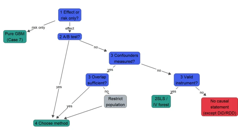
To aid in selecting the appropriate method, a structured decision-making process is proposed. This guide encourages users to proceed sequentially, halting at the first point where a condition cannot be met. The process emphasizes understanding the decision context, the nature of treatment assignment, and crucially, the causal relationships between variables.

Step 1: Defining the Decision and Target Quantity

The initial step involves clarifying the analytical objective. Questions such as "Does the intervention work on average?" or "For whom should we target the intervention?" dictate the target quantity of interest, ranging from the Average Treatment Effect (ATE) to individual-level Conditional Average Treatment Effects (CATE) or rankings of units by their estimated effect.

• Average Treatment Effect (ATE): The average impact of an intervention across the entire population.
• Conditional Average Treatment Effect (CATE): The estimated effect for specific subgroups or individual units based on their characteristics.
• Ranking of Units by Effect: Identifying individuals or entities who are predicted to benefit most from an intervention.
• Risk Assessment (without intervention): Understanding the baseline probability of an undesirable outcome. This is distinct from estimating intervention effects and often addressed by standard predictive models.
• Dose-Response Curve: Estimating how the outcome changes with varying levels or intensity of the intervention. This was not explicitly simulated but is a critical area of advanced causal inference.

Step 2: Understanding Treatment Assignment

The method of treatment assignment is a critical determinant of the appropriate analytical approach.

• Randomized Controlled Trials (RCTs) / A/B Tests: In these scenarios, treatment is assigned randomly, eliminating confounding by pre-treatment variables. This significantly simplifies the estimation process, often allowing for direct comparison of means.
• Observational Data: In contrast, observational studies involve no random assignment. Treatment status is determined by a variety of factors, necessitating careful control for potential confounders to avoid biased estimates.

Step 3: Identification – The Crucial Pre-Modeling Stage

This step is where many causal inference projects falter. It involves understanding the causal relationships between variables and determining which variables must be included in the model to achieve unbiased estimation. Three key terms define these relationships:

• Confounder: A variable that influences both the treatment assignment and the outcome. For example, age might influence whether a customer receives a targeted marketing call (treatment) and also their likelihood of responding to it (outcome). Ignoring confounders leads to attributing their effect to the treatment.
• Mediator: A variable that lies on the causal pathway between the treatment and the outcome. For instance, if a marketing campaign leads to increased website engagement, which in turn drives sales, website engagement is a mediator. Including mediators in the model when interested in the total effect will underestimate the intervention’s true impact.
• Collider: A variable that is influenced by both the treatment and the outcome. Adjusting for a collider can introduce spurious associations between the treatment and the outcome.

The guiding principle is: variables that exist before the treatment and co-determine it, along with the outcome, must be included in the model. Conversely, variables that arise after the treatment and are influenced by it should generally be excluded if the total effect is of interest. This determination is based on domain knowledge, not on data patterns alone.

Step 4: Selecting the Appropriate Method

Based on the insights from the preceding steps, a specific causal inference method can be recommended. The guide presents a decision tree that prioritizes the data situation and the research question.

#	Data Situation	Question	Recommendation	Cross-check	Avoid	Evidence
1	A/B test	Average	Comparison of means. LM (T + X) at most for variance reduction.	—	—	Case 1, 6–8
2	A/B test, little data (a few hundred)	Ranking or effect per unit	Check for effect variation. If none, use average (LM T + X).	Causal forest	T-learner and GBM S-learner	Case 1
3	A/B test, few variables, simple form plausible	Ranking or effect per unit	GLM with T x X.	S-learner, causal forest	Pure risk model	Case 6, 7
4	A/B test, many variables, form unknown	Ranking	S-learner.	Causal forest, R-learner	Double ML and AIPW, pure risk model	Case 8
5	A/B test, many variables, form unknown	Effect per unit	Causal forest. Provides confidence intervals.	R-learner	GLM with T x X or all 2-way interactions	Case 8
6	No randomization; confounders measured, linear	Average	LM (T + X).	Double ML	Naive comparison	Case 2
7	No randomization; confounders measured, nonlinear or unknown	Average	Double ML with GBM.	AIPW, causal forest	LM and S-learner (biased)	Case 3
8	No randomization; confounders measured	Ranking	R- or S-learner.	Causal forest	Pure risk model	Case 9
9	No randomization; confounders measured	Effect per unit	Causal forest.	R-learner	LM/GLM (ATE bias), AIPW (fails in runs)	Case 9
10	No randomization; confounder missing, instrument available	Average	2SLS or Instrumental forest.	Placebo test	All methods without an instrument	Case 5
11	No randomization; confounder missing, no instrument	Any question about the effect	No causal method. Report association with E-value. Exception: DiD, RDD.	—	Any method that outputs an effect number	Case 5

Step 5: Validation and Refinement

After selecting a method, it is crucial to validate its performance. For randomized data, a hold-out set can be used to compare the estimated effects against the simple difference in means. For observational data, the evaluation becomes more complex, relying on sensitivity analyses, placebo tests, and diagnostic checks for model assumptions like overlap.

Step 6: Decision Under Uncertainty

When faced with ambiguity or conflicting results, the principle of parsimony often guides decision-making. Favor the simplest model that adequately explains the data and meets the analytical objectives. More complex methods should only be adopted if they demonstrate clear and significant improvements in performance on validated data.

Methodological Foundations

The core innovation of Causal ML lies in its shift from purely predictive modeling (e.g., predicting Y) to estimating the causal effect of a treatment (T) on Y. This distinction is critical because a model that predicts Y well does not necessarily isolate the effect of T, especially in the presence of confounding. Simulations are essential for evaluating these methods, as they allow for direct comparison against a known "ground truth."

Key Causal Inference Terms

• Potential Outcomes: The hypothetical outcomes for a unit under treatment and control conditions ((Y(1)) and (Y(0))).
• ATE: Average Treatment Effect.
• CATE: Conditional Average Treatment Effect, the effect for units with specific characteristics (x).
• Confounder, Mediator, Collider: Variables that influence causal pathways in specific ways.
• Instrument: A variable that affects treatment assignment but influences the outcome only through the treatment, useful for handling unobserved confounding.
• Effect Modifier: A variable on which the magnitude of the treatment effect depends.

Simulated Scenarios and Findings

The study presents nine distinct simulation cases, categorized into four blocks: Simple World, Variable Selection, Model Flexibility, and Combined Challenges. Each case meticulously details the data generation process, the causal structure (often visualized with Directed Acyclic Graphs – DAGs), and the performance of various methods across key metrics like ATE bias, CATE Root Mean Squared Error (RMSE), and top-30% uplift.

Case Studies Highlight Key Challenges:

• Case 2 (Linear Confounding): Demonstrates that a simple linear model (LM) correctly accounting for a linear confounder significantly outperforms naive comparisons and more complex models that fail to incorporate the confounder.
• Case 3 (Nonlinear Confounding): Underscores the limitations of standard LMs when confounders exhibit non-linear relationships. Here, advanced methods like Double ML and Causal Forests excel by flexibly modeling confounder effects, achieving near-zero ATE bias where LMs fail.
• Case 4 (Mediator Variable): Illustrates a common pitfall where including a mediator (a variable on the causal pathway) drastically underestimates the total treatment effect. This highlights the importance of domain knowledge in defining the causal model.
• Case 5 (Unobserved Confounding): Shows that when critical confounders are unmeasured, standard methods fail. Only the introduction of a valid instrumental variable allows for unbiased estimation.
• Case 6 (Linear Heterogeneity): Reveals that when effects vary linearly with a known variable, a GLM with interaction terms can be more accurate and interpretable than more complex tree-based methods.
• Case 7 (Risk vs. Uplift): A critical scenario for marketing and retention efforts. It shows that targeting based solely on risk prediction is ineffective; methods that explicitly model the treatment effect (like S-learners or GLMs with interaction) are necessary for identifying "persuadables."
• Case 8 (Many Variables): Highlights the advantage of Causal Forests and R-learners when the effect heterogeneity is complex and depends on interactions among many variables, where simpler models struggle to identify the relevant drivers.
• Case 9 (Observational Data + Heterogeneity): A realistic scenario combining confounding and effect modification. Causal Forests and R-learners demonstrate superior performance in accurately estimating both the average effect and individual-level effects, outperforming biased linear models.

Overall Performance and Predictive Accuracy vs. Causal Accuracy

A key insight from the simulations is that predictive accuracy does not equate to causal accuracy. Methods that achieve high predictive performance can be severely biased in their causal estimates, particularly when dealing with unobserved confounding or mediators. The Causal Forest demonstrates its strength in complex scenarios involving unknown interactions and heterogeneous effects, often providing both accurate rankings and magnitudes of effect. However, in simpler settings, well-specified linear models or Double ML can be equally or more effective.

Evaluating Methods Without Ground Truth

In real-world applications, the true causal effect is unknown. The study explores evaluation metrics like R-loss and Qini coefficients, finding that they generally correlate well with true performance in scenarios where identification is sound. However, these metrics cannot detect fundamental issues like unobserved confounding or mediator inclusion. Placebo tests and E-values offer some recourse for assessing sensitivity to unmeasured confounders, but domain knowledge remains the ultimate arbiter of model validity. Confidence intervals, while valuable for quantifying random error, are shown to be unreliable when systematic biases due to flawed identification are present.

Conclusion: When Causal ML Delivers Value

Causal ML methods prove their worth in situations characterized by:

• Non-linear relationships in confounding variables.
• Complex or unknown effect heterogeneity that requires flexible modeling.
• Targeting interventions where identifying individuals likely to benefit is crucial.

They offer little advantage, and can even be detrimental, in scenarios with small sample sizes, linear relationships, correct identification of variables, or when simpler, well-specified models suffice. The research provides a practical guide and extensive simulation evidence to help practitioners navigate the complexities of causal inference and select the most appropriate methods for their specific analytical challenges. The study emphasizes that while advanced algorithms are powerful tools, they must be employed within a rigorous framework of causal reasoning, informed by domain knowledge and careful consideration of the data generation process.