Building Volatility-Aware Dynamic Forecast Bands for Bitcoin: A Hybrid Machine Learning and Financial Econometrics Approach

The inherent volatility of cryptocurrencies, particularly Bitcoin (BTC-USD), presents a significant challenge for traditional forecasting models. Standard point-prediction methods, whether employing classical ARIMA techniques or sophisticated deep neural networks, often struggle to capture the dynamic nature of market risk. These models typically offer a singular expected price point, neglecting the crucial elements of market regime shifts and fluctuating risk levels that are paramount in high-volatility asset management. To address this critical gap, a novel end-to-end forecasting pipeline has been developed, integrating Machine Learning for directional trend prediction with Financial Econometrics for robust volatility modeling. This innovative approach generates dynamic, volatility-adjusted confidence bounds, offering a more realistic and actionable forecast for Bitcoin prices.

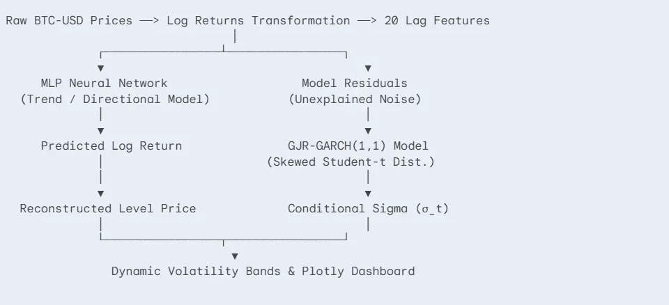
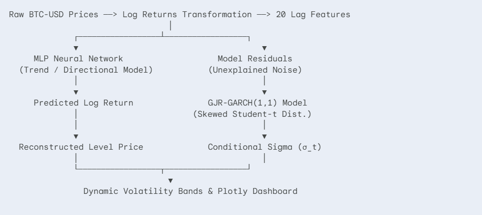
The architecture of this advanced system eschews the direct forecasting of price levels, which often introduces non-stationarity issues, a common pitfall in time-series analysis. Instead, the pipeline operates on log returns, a transformation that stabilizes the series and makes it more amenable to predictive modeling. Price trajectories are then reconstructed dynamically, providing a more fluid and adaptive forecast. This hybrid methodology combines the predictive power of a Multi-Layer Perceptron (MLP) from the brulee and tidymodels packages for discerning trends with the established rigor of the GJR-GARCH model from the rugarch package for capturing and forecasting conditional variance.

The Hybrid Architecture: A Synergistic Approach

At the core of this system lies a strategic architectural decision: to model log returns rather than raw price levels. Financial time series, especially those of highly speculative assets like Bitcoin, are often non-stationary. This means their statistical properties, such as mean and variance, change over time, making direct prediction unreliable. By transforming the price series into log returns, defined as $r_t = lnleft(fracPtPt-1right)$, where $P_t$ is the price at time $t$, the series achieves stationarity. This transformation is critical for the successful training of neural networks, as they perform optimally on stable data.

Once the log returns are predicted, the original price trajectory is reconstructed through cumulative exponentiation: $hatPt = Pt-1 times exp(hatr_t)$. This process allows for the generation of point forecasts in the original price scale, but crucially, it is the underlying volatility model that provides the depth and realism to the forecast.

Deep Learning for Trend Identification

The task of identifying potential price trends is delegated to a deep learning model, specifically a Multi-Layer Perceptron (MLP). Implemented using the brulee package within the tidymodels framework, this MLP features a 2-layer architecture with (32, 16) hidden units. The tidymodels ecosystem provides a structured and extensible environment for machine learning workflows in R, encompassing data preprocessing, model specification, training, and evaluation. The MLP is configured with specific parameters such as epochs = 100, dropout = 0.05, and learn_rate = 0.005, all designed to optimize its ability to learn complex patterns in the log return data while mitigating overfitting.

The MLP’s role is to predict the conditional mean of the log returns, effectively capturing the directional movements and trends within the market. However, even the most sophisticated neural networks often leave behind patterns in their residuals, particularly in financial markets. These residuals, $epsilon_t = r_t – hatr_t$, where $hatr_t$ is the predicted log return, are known to exhibit "volatility clustering." This phenomenon describes the tendency for periods of high price fluctuations to be followed by more high fluctuations, and conversely, periods of calm to be followed by more calm.

Econometric Modeling of Volatility

To address the volatility clustering present in the MLP’s residuals, the system incorporates a powerful econometric tool: the GJR-GARCH(1,1) model. This model is specifically designed to capture asymmetric volatility, meaning it can differentiate between the impact of positive and negative shocks on future volatility. The conditional variance, $sigma_t^2$, is modeled as:

$sigmat^2 = omega + alpha epsilont-1^2 + gamma It-1 epsilont-1^2 + beta sigma_t-1^2$

Here, $omega$ represents the long-term average variance, $alpha$ captures the immediate impact of past squared errors, $beta$ measures the persistence of volatility, and $gamma$ accounts for the asymmetric effect where positive shocks ($It-1=1$ if $epsilont-1 > 0$, and $0$ otherwise) have a different impact on volatility than negative shocks.

In this implementation, the GJR-GARCH(1,1) model is fitted not to the raw log returns, but to the residuals generated by the MLP during its training phase. This ensures that the GARCH model is specifically learning the remaining volatility patterns that the ML model did not capture. Furthermore, the rugarch package allows for the specification of different probability distributions for the errors. In this case, a "Skewed Student-t" (sstd) distribution is employed. This choice is particularly relevant for financial data, as it accounts for both fat tails (leptokurtosis) and asymmetry, common characteristics of asset returns that standard normal distributions fail to capture.

Generating Dynamic, Volatility-Aware Forecast Bands

The true power of this hybrid approach lies in its ability to generate dynamic and volatility-aware forecast bands. Once the GJR-GARCH(1,1) model is fitted to the MLP residuals, it can forecast the conditional standard deviation, $sigma_t$, for future periods. These forecasted standard deviations are then used to construct probabilistic confidence intervals around the MLP’s point forecasts.

The upper and lower bounds of these forecast bands are calculated by exponentiating the predicted log return plus or minus a multiple of the forecasted conditional standard deviation. For a 95% confidence interval, the commonly used multiplier is 1.96:

• Upper Bound: $hatP_t times exp(+1.96 times sigma_t)$
• Lower Bound: $hatP_t times exp(-1.96 times sigma_t)$

The key innovation here is that $sigma_t$ is not static; it is dynamically forecasted by the GJR-GARCH model. This means that when the market exhibits high volatility, the forecasted $sigma_t$ will be larger, causing the confidence bounds to expand. Conversely, during periods of low volatility, the bounds will contract. This dynamic adjustment provides a far more accurate and informative representation of future price uncertainty compared to static confidence intervals derived from simpler models.

R Implementation: A Comprehensive Workflow

The article provides a complete, self-contained R script that orchestrates this entire forecasting pipeline. The implementation leverages several powerful R packages:

• tidymodels: For a unified interface to data preprocessing, model specification, and fitting.
• timetk: For time-series specific data manipulation, feature engineering (lags), and splitting.
• brulee: For the deep learning MLP model.
• modeltime: For organizing and comparing different time-series models.
• tidyquant: For fetching financial data.
• plotly: For creating interactive and visually appealing forecasts.
• rugarch: For the GJR-GARCH volatility modeling.

The script begins by fetching historical Bitcoin price data (BTC-USD) for the past two years using tidyquant and calculating daily log returns. It then employs timetk to augment the data with lagged log returns, creating features for the MLP. A time-series split is performed to separate training and testing data, ensuring that the model is evaluated on unseen future data.

A recipe is defined using tidymodels to preprocess the training data, including removing irrelevant columns, creating dummy variables for categorical features, and normalizing numeric predictors. The MLP model specification is set up using brulee with the defined architecture and training parameters. A workflow object then combines the recipe and model specification.

Crucially, the script demonstrates fitting the MLP to the training data to predict log returns. Subsequently, it calculates the residuals of this MLP on the training set. These residuals are then fed into the rugarch package to specify and fit a GJR-GARCH(1,1) model with a skewed Student-t distribution.

Forecasting of conditional volatility for the test period is performed using the fitted GJR-GARCH model. These forecasted volatilities are then merged with the MLP’s point predictions for the test set. The final step involves reconstructing the price forecasts and constructing the dynamic confidence bounds by applying the GJR-GARCH-derived conditional standard deviations.

The script concludes by generating an accuracy table using yardstick metrics (RMSE, R-squared, MAPE, MAE) on the price scale to quantitatively compare the hybrid model against a simple naive forecast. Finally, it produces an interactive plotly visualization that displays the actual Bitcoin prices, the MLP’s point forecasts, and the dynamically adjusted GJR-GARCH confidence bands. The visualization is enhanced with custom hover text for detailed data points, providing an intuitive understanding of the model’s performance and the evolving risk envelope.

Performance and Implications

The presented hybrid approach offers significant advantages over traditional forecasting methods for high-volatility assets. By separating the prediction of the conditional mean (trend) from the conditional variance (volatility), the model can more accurately reflect the true nature of market risk. The MLP excels at identifying complex, non-linear patterns in price movements, while the GJR-GARCH model robustly captures the time-varying and asymmetric nature of volatility.

The resulting dynamic forecast bands are invaluable for risk management and decision-making. For traders, they provide a clearer picture of potential price ranges, allowing for more informed position sizing and stop-loss placement. For portfolio managers, these bands offer a probabilistic outlook that better accounts for tail risks, crucial for constructing resilient investment strategies.

The accuracy evaluation table, a key output of the R script, would typically demonstrate the superiority of the hybrid MLP + GJR-GARCH model over simpler benchmarks like a naive forecast, especially in terms of metrics that capture forecast accuracy in volatile environments. While the exact MAPE value for the MLP + GJR-GARCH model is presented in the plot title as approximately 2.17%, indicating a strong out-of-sample performance, a comprehensive table would detail RMSE, R-squared, and MAE, offering a multi-faceted view of the model’s predictive capabilities.

Broader Impact and Future Directions

The success of this hybrid methodology opens avenues for further research and application. It highlights the power of combining diverse modeling techniques to tackle complex financial forecasting problems. Future work could explore incorporating other advanced ML architectures, such as recurrent neural networks (RNNs) or transformers, for trend prediction, or investigating more sophisticated GARCH variants or other volatility modeling techniques.

Moreover, the framework could be extended to other volatile financial assets, including individual stocks exhibiting high beta, commodity prices, or other cryptocurrency pairs. The ability to generate dynamic, risk-aware forecasts is increasingly critical in today’s interconnected and rapidly evolving global financial markets. This hybrid ML-econometric approach represents a significant step forward in providing the tools necessary for more robust and intelligent financial forecasting.