Permute Introduces Powerful New Tools for Advanced Permutation Testing in R

The R statistical programming language, a cornerstone for data analysis and scientific research, has seen a significant advancement in its permutation testing capabilities with the introduction of new functionalities in the permute package. In a recent development, the package has unveiled two powerful helper functions, permutations() and permutator(), designed to streamline the process of generating and applying permutations for robust statistical inference. These tools are poised to enhance the efficiency and flexibility for researchers conducting permutation tests, a non-parametric method crucial for hypothesis testing when assumptions of traditional parametric tests are not met.

The latest iteration of the permute package, available in its development version, offers these innovative functions to facilitate the second phase of permutation test construction: the application of generated permutations to data. While the previous installment of the permute package focused on ordered set partitions and formula interfaces for plots and blocks, this update directly addresses the practical application of shuffled data. The permutations() function provides direct access to shuffled values, while permutator() generates a callable function that systematically delivers the next set of observation indices upon each invocation. Both functions leverage the same underlying permutation machinery, enabling researchers to implement permutation tests using slightly different, yet equally effective, methodological approaches.

To access these cutting-edge features, users are advised to install the development version of the permute package from the author’s R-universe repository. The installation process is straightforward:

install.packages("permute", repos = c(
  "https://gavinsimpson.r-universe.dev",
  "https://cloud.r-project.org"
))

Unpacking the Power: A Case Study with PlantGrowth Data

To illustrate the practical utility of these new functions, the development team has employed the well-known PlantGrowth dataset, a standard inclusion in R’s base distribution. This dataset meticulously records the dried weights of plants subjected to three distinct conditions: a control group and two treatment groups (trt1 and trt2).

Initial exploratory analysis of the PlantGrowth data reveals notable differences in mean plant weights across the groups:

library("permute")
data(PlantGrowth, package = "datasets")

aggregate(weight ~ group, data = PlantGrowth, FUN = mean)

The output of this aggregation is as follows:

  group weight
1  ctrl  5.032
2  trt1  4.661
3  trt2  5.526

These mean differences are visually apparent, but the critical question for statistical inference is whether these observed variations are statistically significant, or if they could reasonably arise by chance under a null hypothesis of no treatment effect. To address this, the permute package facilitates the use of an overall F statistic derived from a linear model. This statistic quantifies the ratio of variance between groups to variance within groups, serving as a measure of the overall difference in plant weights across the experimental conditions. Larger F statistics indicate greater divergence between group means relative to the inherent variability within each group.

A specialized function, f_stat, has been defined to encapsulate this F-statistic calculation:

f_stat <- function(weight, group) 
  fit <- lm(weight ~ group)
  unname(summary(fit)$fstatistic[["value"]])


observed <- with(PlantGrowth, f_stat(weight, group))
print(observed)

The result of this calculation, representing the observed F statistic from the original data, is:

[1] 4.846088

This observed F statistic provides a benchmark against which the results from permuted datasets will be compared. The permutation test operates under the null hypothesis that the plant weights are exchangeable across the treatment groups. In essence, it assumes that the observed differences in weights are not attributable to the specific treatments but could have occurred randomly if the group labels were reassigned. The core of the permutation test involves shuffling these weights among the group labels to generate a null distribution of the F statistic.

Direct Shuffling with permutations()

The permutations() function offers a direct route to obtaining shuffled datasets. Unlike the more traditional shuffleSet() function, which typically returns permuted indices, permutations() directly yields the shuffled values themselves. This means that for each generated permutation, the function returns a vector containing the permuted plant weights.

To control the number of permutations, the how() function is utilized. For this demonstration, 9,999 permutations are requested:

ctrl <- how(nperm = 9999)

set.seed(42) # For reproducibility
shuffled <- permutations(PlantGrowth$weight, control = ctrl)

The shuffled object is structured such that each row represents a unique permutation of the original PlantGrowth$weight vector. The columns correspond to the original positions of the observations. This structure allows for straightforward pairing with the unchanged PlantGrowth$group vector. To provide a glimpse into the generated permutations, the first few values from the first three shuffled rows are displayed:

# Displaying a subset for illustration
print(as.matrix(shuffled)[seq_len(3), seq_len(5)])

The output reveals the scrambled nature of the weights:

     [,1] [,2] [,3] [,4] [,5]
[1,] 6.03 4.50 4.17 5.37 5.14
[2,] 4.81 5.87 5.12 5.29 4.53
[3,] 5.14 4.53 4.50 4.17 6.03

These permuted weight vectors are then used to recalculate the F statistic for each permutation. The apply() function is adept at iterating through the rows of the shuffled object and applying the f_stat function:

null_values <- apply(shuffled, 1, f_stat, group = PlantGrowth$group)

The resulting null_values vector constitutes the empirical null distribution of the F statistic under the assumption of no treatment effect. The p-value is then computed as the proportion of these permuted F statistics that are equal to or greater than the observed F statistic. A small tolerance (tol) is incorporated to account for potential minor numerical discrepancies arising from the model fitting process:

tol <- sqrt(.Machine$double.eps)
p_value <- (1 + sum(null_values >= observed - tol)) /
  (length(null_values) + 1)

print(c(F = observed, p_value = p_value))

The calculated p-value and observed F statistic are:

       F  p_value 
4.846088 0.014200 

This p-value of approximately 0.0142 suggests that under the null hypothesis, there is about a 1.42% chance of observing an F statistic as extreme as, or more extreme than, the one calculated from the original data. This provides statistical evidence to reject the null hypothesis, indicating that there are significant differences in plant weights among the treatment groups.

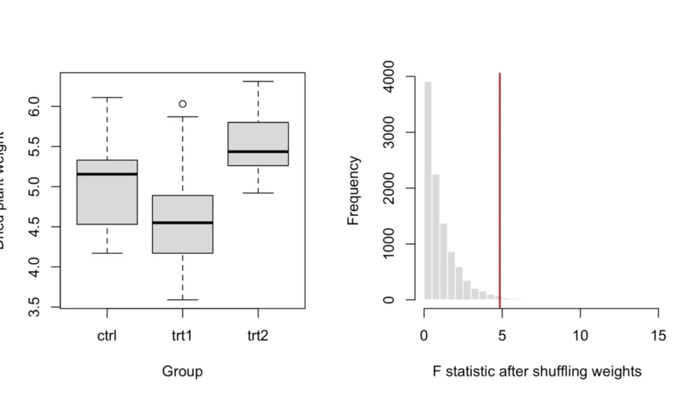
Visualizing the results further solidifies this conclusion. A boxplot of the original plant weights by group, alongside a histogram of the permuted F statistics, illustrates the position of the observed F statistic within the null distribution:

old_par <- par(mfrow = c(1, 2))
boxplot(weight ~ group, data = PlantGrowth,
        xlab = "Group", ylab = "Dried plant weight",
        col = "grey85")
hist(null_values, breaks = 40, main = "",
     xlab = "F statistic after shuffling weights",
     col = "grey85", border = "white")
abline(v = observed, col = "firebrick", lwd = 2)
par(old_par)

The accompanying figure clearly shows the observed F statistic positioned in the right tail of the permutation distribution, reinforcing the statistical significance of the observed treatment effects. The estimation of the p-value from random permutations means that slight variations can occur with different random seeds or numbers of permutations.

It is important to note that permutations() operates on atomic vectors. If a factor is provided, it returns shuffled character labels. The function adheres to the standard shuffleSet() conventions regarding checks and complete enumeration, meaning the actual number of returned rows might differ from the requested number if the permutation space is small. Users should always base subsequent calculations on the size of the returned object.

Iterative Permutation Generation with permutator()

For scenarios where a more iterative approach is preferred, such as within a loop for complex model fitting or progress tracking, the permutator() function emerges as a highly valuable tool. This function generates another function, and each subsequent call to this generated function yields the next permutation of observation indices.

To maintain consistency with the previous demonstration, the random seed is reset:

set.seed(42)
next_perm <- permutator(nrow(PlantGrowth), control = ctrl)

# Initialize a numeric vector to store permuted F statistics
null_iter <- numeric(attr(next_perm, "nperm"))

# Loop through each permutation
for (b in seq_along(null_iter)) 
  i <- next_perm() # Get the next set of indices
  # Calculate F statistic using the permuted indices
  null_iter[b] <- f_stat(PlantGrowth$weight[i], PlantGrowth$group)

In this loop, i represents the indices for the current permutation. PlantGrowth$weight[i] effectively shuffles the weights according to these indices. The attr(next_perm, "nperm") attribute provides the total number of permutations generated, which is used to pre-allocate the null_iter vector for efficiency.

A key characteristic of iterators is their statefulness. Once all permutations have been exhausted, subsequent calls to next_perm() will return NULL. This prevents accidental reprocessing or off-by-one errors.

To verify the consistency of the two approaches, a direct comparison of the generated F statistics is performed:

all.equal(null_values, null_iter)

The result, TRUE, confirms that both methods produced identical F statistics, as expected given the identical underlying permutation sets and experimental design. The p-value calculation from the null_iter results yields the same outcome:

p_iter <- (1 + sum(null_iter >= observed - tol)) /
  (length(null_iter) + 1)

print(c(values = p_value, iterator = p_iter))

The output is:

  values iterator 
  0.0142   0.0142 

It is worth noting that permutator() generates and stores the entire permutation matrix internally upon initialization. While it dispenses rows sequentially, it does not employ lazy generation or eliminate the memory requirement for storing the index matrix.

Reusing and Managing Permutation Sets

The flexibility of permutator() extends to the ability to pass an existing index matrix. This is particularly useful when multiple analyses require the application of the exact same set of permutations or when one wishes to revisit a previously generated and saved set of permutations.

set.seed(42)
indices <- shuffleSet(nrow(PlantGrowth), control = ctrl) # Generate indices first

next_perm <- permutator(perms = indices) # Create iterator from existing indices
i <- next_perm()
print(head(PlantGrowth$weight[i]))

The output shows the first few permuted weights based on the provided indices:

[1] 6.03 4.50 4.17 5.37 5.14 6.11

Crucially, creating a new iterator over the same indices matrix will restart the sequence from the beginning:

replay <- permutator(perms = indices)
identical(i, replay())

This yields TRUE, confirming that a new iterator begins anew. Users can supply either the perms argument or the generation arguments (like n, nset, and control). The matrix provided to perms must contain observation indices, similar to those produced by shuffleSet(). The shuffled weight vectors generated by permutations() are not directly interchangeable with this matrix.

Conclusion and Future Directions

The introduction of permutations() and permutator() in the permute package marks a significant step forward in the R ecosystem for statistical permutation testing. For straightforward analyses involving a single vector and a concise calculation, permutations() combined with apply() offers an elegant and efficient solution. When the analytical workflow naturally lends itself to loops, or when the need arises to reuse specific sets of permutations, permutator() proves to be an invaluable asset.

Both functions maintain the established workflow of defining permutation designs using how(), ensuring that the same robust framework extends to restricted permutation designs when necessitated by the data or research question. The comprehensive package manual, available at the provided link, offers in-depth details and further examples. The developers encourage user feedback and contributions through the project’s issue tracker, fostering a collaborative environment for the continuous improvement of these powerful statistical tools. The implications for researchers are substantial, promising more efficient, flexible, and rigorous hypothesis testing across a wide array of scientific disciplines.